Euler integration of kinematic differential equations for position and orientation

We can integrate kinematic differential equations to determine both 1) where an object will be and 2) what orientation it will have after a specified amount of time. In this post I describe the mathematical proceedure, and implement the solution in Python.

Euler Integration

Euler integration is a 1^st order initial value numerical procedure for solving ordinary differential equations (ODEs). The method can be used to approximate the position/orientation of an object after a period of time, given the initial degrees of freedom, and their 1^st derivatives (i.e. dynamics are not considered). The error in the approximation is proportional to the size of the time step used. For our problem we would like to determine both orientation and position, where angular velocity and linear velocity are specified (their 1^st derivatives).

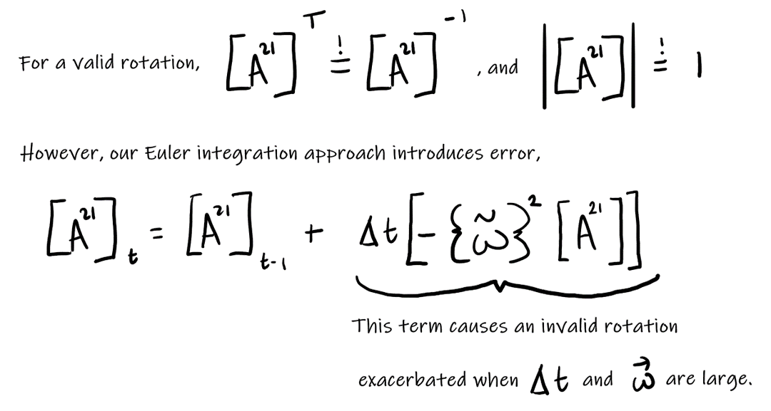
The Euler integration equation for the orientation is apparent, however, the relationship between the angular velocity vector and the 1st time derivative of the rotation matrix is not.

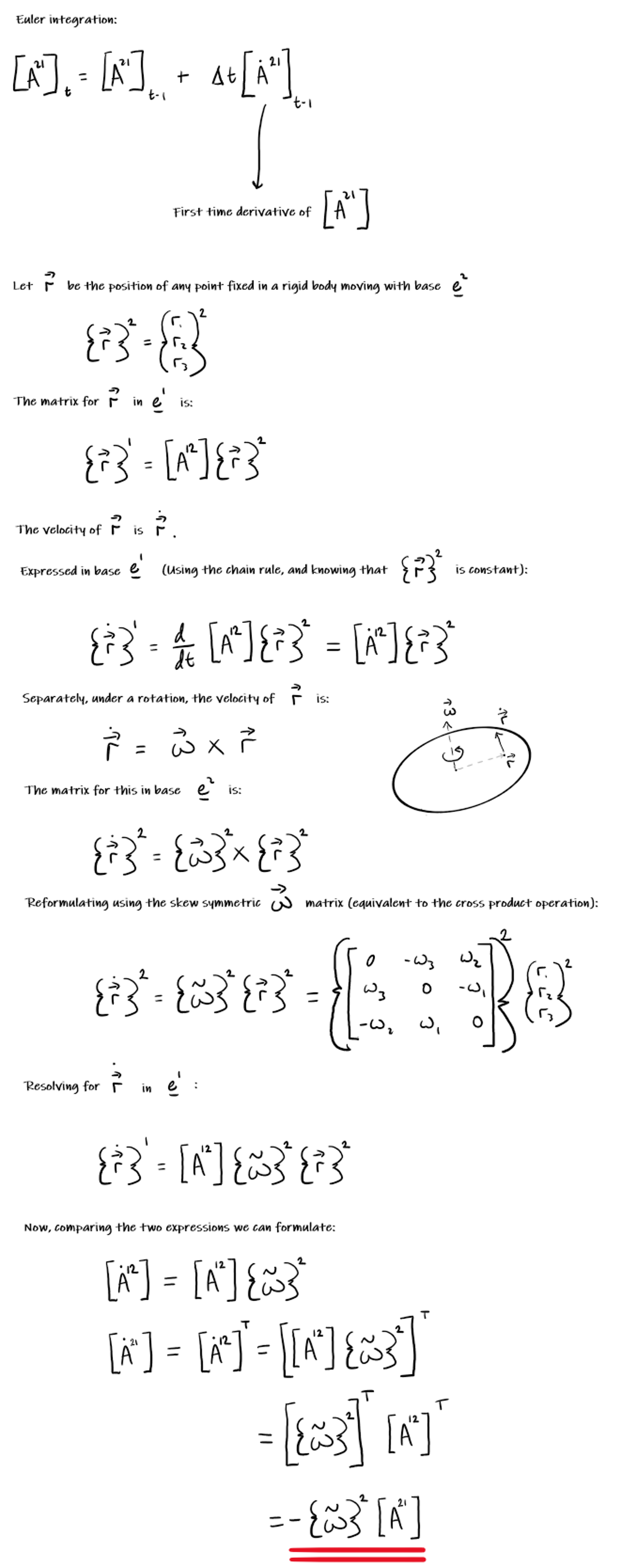
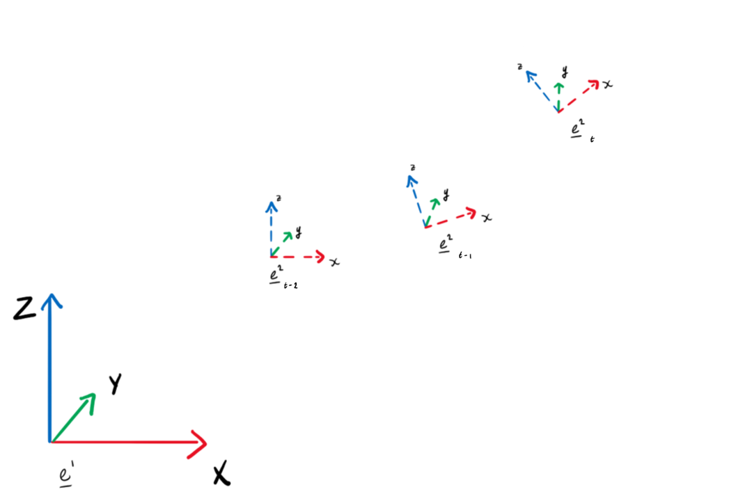
The angular velocity is constant, and acts in the local coordinate system:

We are modelling the motion of a self-propelled object, so we specify the linear velocity in the local coordinate system:

Implementation

I have impelemented Euler integration for both position and orientation of an object in a single function with intitial values, derivatives, end time, and time step as inputs (EulerInt(A0,ω,r0,v,t_step,t_end)).

Note that for a valid rotation the rotation matrix must be 1) orthogonal and 2) have a determinant of 1. However the Euler integration approach introduces error.

Therefore I have implemented a correction term (correction_matrix) as described here, and a function to check validity (isRotationMatrix(M) where a tolerance of 1e-3 is used due to floating-point error).

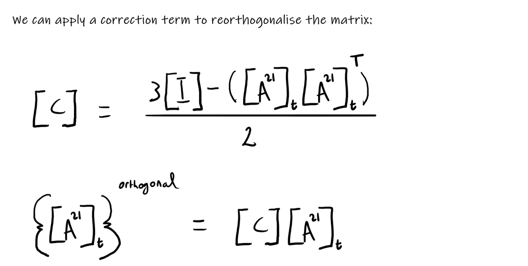
Without this correction matrix the solution becomes invalid, i.e. the rotation matrix becomes non-orthogonal (indicated by the local coordinate system axes no longer being mutually perpindicular), and the determinant no longer equalling 1 (indicated by axes no longer being unit vectors). These errors propagate over time.

Without correction term	With correction term

def isRotationMatrix(M):
    """ Checks whether a rotation matrix is orthogonal, and has a determinant of 1 (tolerance of 1e-3)"""
    tag = False
    I = np.identity(M.shape[0])
    check1 = np.isclose((np.matmul(M, M.T)), I, atol=1e-3)
    check2 = isclose(np.linalg.det(M),1,abs_tol=1e-3)
    if check1.all()==True and check2==True: tag = True
    return tag

def SkewSym(a):
    """ Converts a 1x3 vector to a 3x3 skew symmetric matrix"""
    a_tilda = np.array([[0, -a[2], a[1]],
                        [a[2], 0, a[0]],
                        [-a[1], a[0], 0]])
    return a_tilda

def RevSkewSym(a_tilda):
    """ Converts a 3x3 skew symmetric matrix to a 1x3 vector"""
    if a_tilda[0][0] != 0 or a_tilda[1][1] != 0 or a_tilda[2][2] != 0:
        sys.exit('Error: Matix is not skew symmetric')
    a = np.array([a_tilda[1][2], a_tilda[0][2], a_tilda[1][0]])
    return a

def EulerInt(A0,ω,r0,v,t_step,t_end):
    """ Performs Euler Integration to determine position and velocity given initial conditions, 1st derivatives, time step, and end time"""
    At=A0
    Ats=[]
    rt=r0
    rts=[]
    ω_tilda = SkewSym(ω)
    for t in range(int(t_end/t_step)):
        ω = At @ RevSkewSym(ω_tilda)
        ω_tilda = SkewSym(ω)
        At = At + t_step*(-ω_tilda @ At)
        correction_matrix = (3*np.array([[1, 0, 0],[0, 1, 0],[0, 0, 1]]) - (At @ At.T))/2 # correction matrix to ensure that the rotation matrix is orthogonal
        At = correction_matrix @ At
        if isRotationMatrix(At)==False:
            sys.exit('Error: Chosen integration time step is too large - try a smaller value (generally a step of <=1e-2 is recommended)')
        Ats.append(At)
        rt = rt + t_step*(At@v)
        rts.append(rt)
    return Ats,rts

The full code is available here.