
Solution space for mapping serial kinematic chains
Mapping kinematic chains
Kinematic chains can be described as a hierarchical system of links and joints. Kinematic chains are described by 1) the locations and orientations of each of the joints, and 2) the heirarchy of the joints in the system. In this post I develop a method for calculating the solution space for mapping one serial open kinematic chain (i.e. a chain with no branches and no looping) (a) to another (b), where the latter does not contain any information on joint orientations. The chains must have the same number of joints and the same joint heirarchy, but may have differing and disproportional link lengths.
Vector mapping
In a previous post, I described how in SO(3) an infinite number of rotation matrices, or Euler/Screw axis-angle combinations can be applied to map one vector (a) onto another vector (b). However, the solution space is constrained such that the Euler/Screw axis must lay on the plane that bisects the vectors.
For more information see my blog post: ‘Non-uniqueness of the Euler axis in vector mapping’
If we assign an initial local coordinate system to vector a, for example, if we set it to be aligned with the global coordinate system then we can see the Euler axis-angle solution space for reorientation of this local coordinate system.
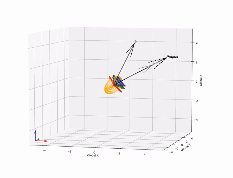
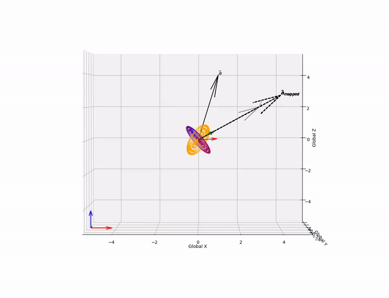
Alternatively, we can choose a simpler joint orientation, with an initial local coordinate system for vector a where the local y-axis (green) is alligned with the vector. In this case, the solution space is more easily visualised.
Definining a kinematic chain and applying forward kinematics
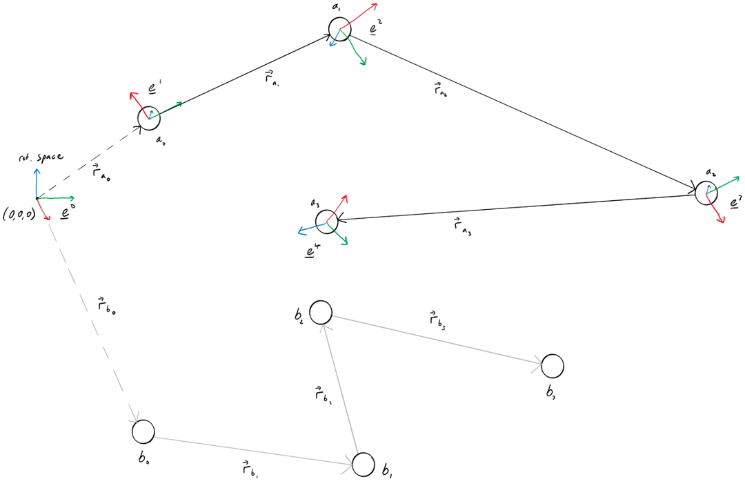
We can define a serial open kinematic chain ‘a’ using a parent-child convention, where the degrees of freedom (DOFs) of child joints are expressed with respect to the parent joint DOFs. I.e. the position of the child joint is expressed as a vector in the coordinate system of the parent joint, and the orientation of the child joint is expressed as a rotation matrix which specifies the orientation of the child joint wrt. the parent joint’s orientation. This is the conventional approach for defining kinematic chains because it allows for various kinematic and dynamic operations to be performed.
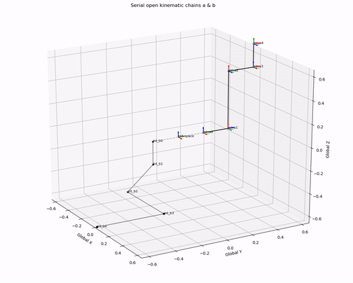
Firstly, we can consider a serial open kinematic chain, where the joints are arranged in series with no forking (i.e. all joints in the chain have a maximum of one child joint), where joint a0 is the root joint which is connected to the reference space. See here for a brief overview of some relevant theory for the 3D rotation group.
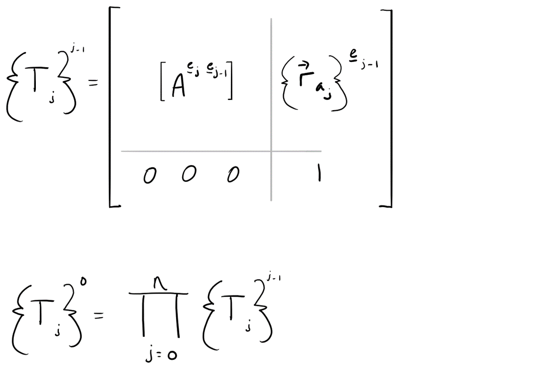
We can use this information to calculate the joint positions and orientations in the global coordinate system i.e. perform forward kinematics. The most common method for this is the modified D-H convention, which allows for a compact expression for all 6 joint DOFs as a 4x4 transformation matrix. Where the coefficients contain information on the relative position and orientation of joint j wrt. joint j-1. The forward kinematics operation is simply a serial multiplication of all transformation matrices on the path to joint j.
Using this knowledge we can programatically define a kinematic chain and plot it in the global coordinate system using forward kinematics.
chain_a.append(['jnt_a0', np.array([[ 1, 0, 0, 0],
                                    [ 0, 1, 0, 0.2],
                                    [ 0, 0, 1, 0],
                                    [ 0, 0, 0, 1]])])
chain_a.append(['jnt_a1', np.array([[ 0, 1, 0, 0],
                                    [ 0, 0, 1, 0.2],
                                    [ 1, 0, 0, 0],
                                    [ 0, 0, 0, 1]])])
chain_a.append(['jnt_a2', np.array([[ 1, 0, 0, 0.5],
                                    [ 0, 0, 1, 0],
                                    [ 0, 1, 0, 0],
                                    [ 0, 0, 0, 1]])])
chain_a.append(['jnt_a3', np.array([[ 0, 0, 1, 0],
                                    [ 1, 0, 0, 0.2],
                                    [ 0, 1, 0, 0],
                                    [ 0, 0, 0, 1]])])
chain_a.append(['jnt_a4', np.array([[ 1, 0, 0, 0],
                                    [ 0, 0, 1, 0],
                                    [ 0, 1, 0, 0.2],
                                    [ 0, 0, 0, 1]])])
In order to perform kinematic operations on the chain we must also specify its heirarchical structure using a directed graph.
dir_graph = {0: [1],
             1: [2],
             2: [3],
             3: [4]}
For implementation of forward kinematics we must use the directed graph to define the path for each joint (i.e. create a list of all joints on the path from the root joint).
def jnt_path(graph, start, end, path=[]):
    """ list all joints on the path to a specified joint"""
    path = path + [start]
    if start == end:
        return path
    if not start in graph:
        return None
    for node in graph[start]:
        if node not in path:
            newpath = jnt_path(graph, node, end, path)
            if newpath: return newpath
    return None
The forward kinematics solution first defines the reference space to be at (0,0,0) with an identity matrix orientation, then reads in the locally defined joint DOFs for each joint and sequentially calculates the global DOFs along the path to the joint.
def FK_MDH(chain,dir_graph):
    """ perform forward kinematics to to convert joint orientations and position vectors into the global coordinate system"""
    oris=[]
    poss=[]
    for i in range (len(chain)):
        path = jnt_path(dir_graph, 0, i)
        T=np.array([[ 1, 0, 0, 0],
                    [ 0, 1, 0, 0],
                    [ 0, 0, 1, 0],
                    [ 0, 0, 0, 1]])
        for j in path:
            T= T @ chain[j][1]
            pos=np.array([T[0][3],T[1][3],T[2][3]])
            ori=np.array([[T[0][0],T[0][1],T[0][2]],[T[1][0],T[1][1],T[1][2]],[T[2][0],T[2][1],T[2][2]]])
        oris.append(ori)
        poss.append(pos)
    return oris, poss
Plotting the kinematic chain in the global coordinate sysem:
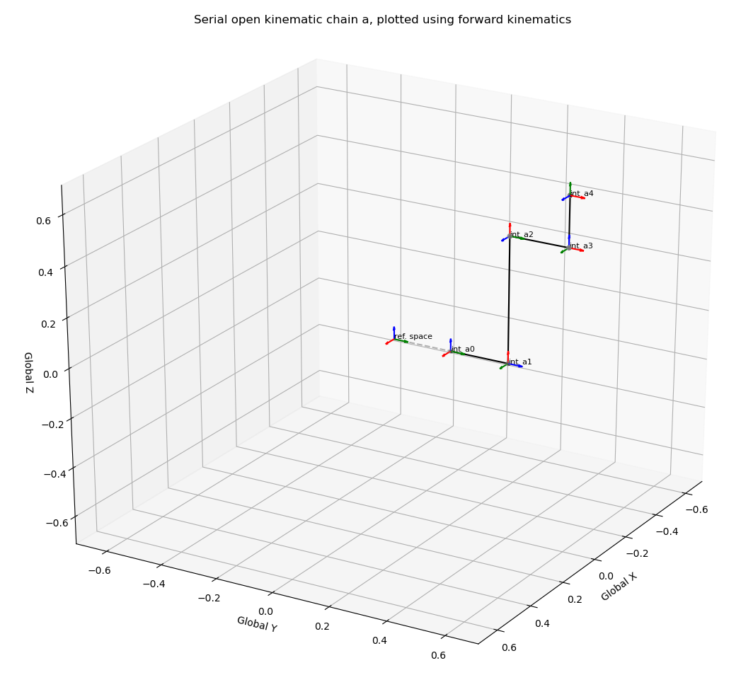
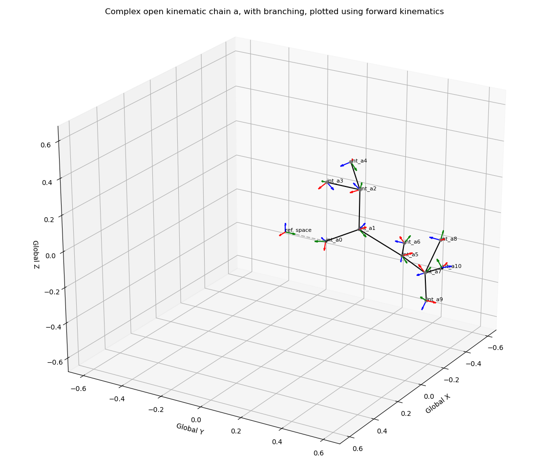
Since we use the path to each joint from the directed graph, this approach also works for more complex open kinematic chains with branching (i.e. where joints may have multiple children).
The usefulness of defining a kinematic chain in this manner can be seen if we decide to edit or reorient our kinematic chain. For example, if I would like to reorient a joint in the chain, it makes physical sense to apply the rotation in the local coordinate system, i.e. if you rotate your elbow, the rotation is kinematically constrained to occur about a fixed axis defined in the local coordinate system (usually chosen to be a cardinal axis). Furthermore, the orientation change you make to the elbow should reorient downchain joints to the same extent (can be applied using forward kinematics).
For example, if I reorient jnt_a0, and joint_a5 in the example above by 45 degrees about their local x axes (shown in red), the positions and orientations of downchain joints are transformed appropriately:
| jnt_a0 | jnt_a5 |
|---|---|
 |
 |
For practical reasons, currently I am not using a modified D-H convention. I use a more explicit approach for the kinematic chain mapping method, i.e. keeping rotation matrices and vectors separate in forward kinematics operations.
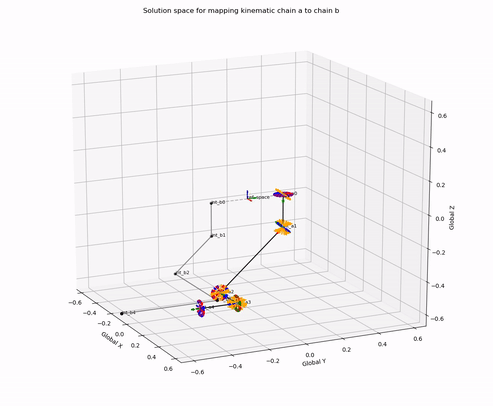
Solution space for mapping kinematic chains
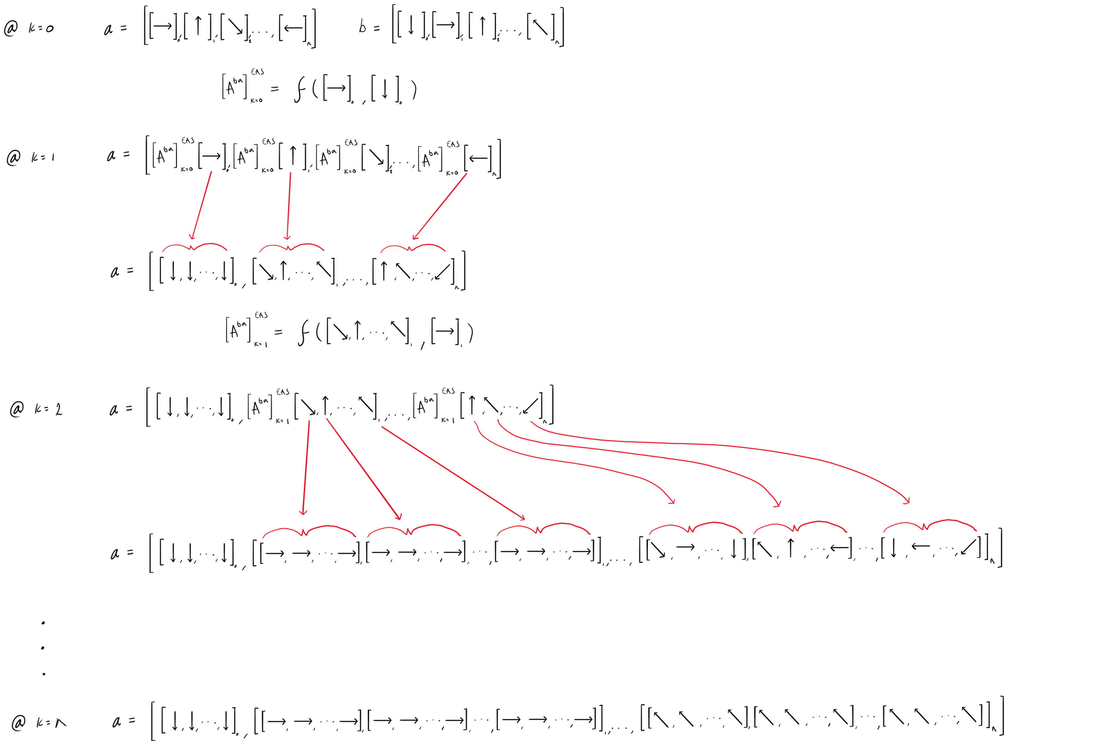
The goal is to use kinematics knowledge to extend the vector mapping method I previously developed for use on a kinematic chain. Specifically, I would like to develop a method for calculating the discretised solution space for mapping one kinematic chain (a) to another (b), where the latter does not contain any information on joint orientations. The chains must have the same number of joints and the same joint heirarchy, but may have differing and disproportional link lengths. This will require a kinematical approach involving sequential calculations of the Euler axis-angle solution space for each joint throughout the chain. The problem is complicated by the fact that the Euler axis-angles applied in upchain joints affect the joint orientations and the resulting solution spaces for mapping downchain vectors.
Step 1: The vector mapping method below requires us to transform chains a and b such that the current joint ak, and bk are at the origin. i.e. first apply this to the root joints a0, and b0.
Step 2: Determine the Euler axis-angle solution space for mapping vector a to vector b (see detailed formulation here).
Step 3: Perform forward kinematics on downchain joints in chain a, including all possible transformations resulting from the joint’s Euler axis-angle solution space.
Step 4: Repeat steps 1 to 3 for each joint in the chain.
The process can be visualised as follows for joints k= [0, n], where a list of vectors for a and b are input sequentially into the vector mapping function, and the output rotation matrices in the solution space are applied to vectors downchain in a.
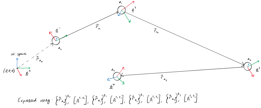
We can use the serial open kinematic chain defined previously, and define chain b. We can do so in either the conventional form for kinematic chains, or simply as positions in the global coordinate system. I have chosen to define it in the conventional form, but the solution only considers vectors in the global coordinate system.
We must define our vector mapping method which will be called upon sequentially throughout the mapping process.
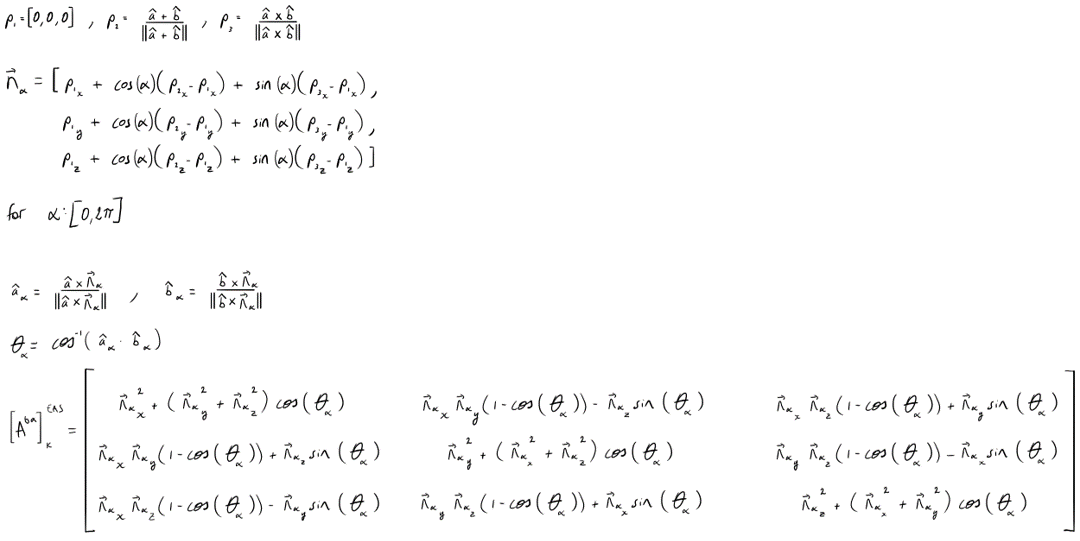
def Vector_mapping_Euler_Axis_Space(vec1, vec2):
    """ Calculate all rotation matrices that map vector a to align with vector b"""
    a, b = (vec1 / np.linalg.norm(vec1)), (vec2 / np.linalg.norm(vec2))
    p1 = np.array([0,0,0])
    p2 = b / np.linalg.norm(b) + (a / np.linalg.norm(a))
    p3 = np.cross(a, b) / np.linalg.norm(np.cross(a, b))
    n=[]
    # create a list of candidate Euler axes (discritised to 1 degree)
    for i in range(0,360,1):
        Φ=np.radians(i)
        x_Φ=p1[0]+np.cos(Φ)*(p2[0]-p1[0])+np.sin(Φ)*(p3[0]-p1[0])
        y_Φ=p1[1]+np.cos(Φ)*(p2[1]-p1[1])+np.sin(Φ)*(p3[1]-p1[1])
        z_Φ=p1[2]+np.cos(Φ)*(p2[2]-p1[2])+np.sin(Φ)*(p3[2]-p1[2])
        n_Φ=[x_Φ,y_Φ,z_Φ]
        n.append(n_Φ / np.linalg.norm(n_Φ))
    # project vectors to form a cone around the Euler axis, and determine required angle for mapping
    rotation_matrices=[]
    Euler_axes=[]
    Euler_angles=[]
    for i in range(len(n)):
        Euler_axes.append(n[i])
        a_Φ, b_Φ = (np.cross(a,n[i]) / np.linalg.norm(np.cross(a,n[i]))), (np.cross(b,n[i]) / np.linalg.norm(np.cross(b,n[i])))
        θ = np.arccos(np.dot(a_Φ,b_Φ))
        θ = θ*np.sign(np.dot(n[i], np.cross(a_Φ,b_Φ)))
        Euler_angles.append(θ)
        if θ != θ: # if θ is NaN
            rotation_matrices.append(np.array([[ 1, 0, 0],
                                               [ 0, 1, 0],
                                               [ 0, 0, 1]]))
        else:
            rotation_matrices.append(np.array([[n[i][0]**2+(n[i][1]**2+n[i][2]**2)*(np.cos(θ)),n[i][0]*n[i][1]*(1-np.cos(θ))-n[i][2]*np.sin(θ),n[i][0]*n[i][2]*(1-np.cos(θ))+n[i][1]*np.sin(θ)],
                                        [n[i][0]*n[i][1]*(1-np.cos(θ))+n[i][2]*np.sin(θ),n[i][1]**2+(n[i][0]**2+n[i][2]**2)*(np.cos(θ)),n[i][1]*n[i][2]*(1-np.cos(θ))-n[i][0]*np.sin(θ)],
                                        [n[i][0]*n[i][2]*(1-np.cos(θ))-n[i][1]*np.sin(θ),n[i][1]*n[i][2]*(1-np.cos(θ))+n[i][0]*np.sin(θ),n[i][2]**2+(n[i][0]**2+n[i][1]**2)*(np.cos(θ))]]))

    return Euler_axes, Euler_angles, rotation_matrices
Next, I apply my method for a discretised Euler axis-angle solution space for each joint in the kinematic chain.
def Serial_open_chain_mapping(chain_a, chain_b, dir_graph): # Consider renaming Could more aptly be described as a modified forward kinematics approach?
    """ perform inverse kinematics to map a serial kinematic chain a (an open chain without forking) to chain b, which must have the same directed graph"""
    ori_a, pos_a = FK_MDH(chain_a,dir_graph)
    _, pos_b = FK_MDH(chain_b,dir_graph)

    pos_a= pos_a - chain_a[0][2]
    pos_b= pos_b - chain_b[0][2]

    #convert directed graph for use in nx
    dir_graph = nx.DiGraph(dir_graph)

    repos_a_EAS=[]
    reori_a_EAS=[]
    Euler_axis=[]
    Euler_axes=[]

    for i in range(1,360,1):
        reori_a=copy.deepcopy(ori_a)
        repos_a=copy.deepcopy(pos_a)
        Euler_axis=[]
        for j in range(len(chain_a)):
            downchain = list(nx.nodes(nx.dfs_tree(dir_graph, j))) # list of index values for j and all joints down chain
            if j < len(chain_a)-1:
                ROTM= Vector_mapping_Euler_Axis_Space(repos_a[j+1]-repos_a[j], pos_b[j+1]-pos_b[j])[2][i]
                Euler_axis.append(Vector_mapping_Euler_Axis_Space(repos_a[j+1]-repos_a[j], pos_b[j+1]-pos_b[j])[0][i])
            for k in range(len(downchain)):
                if downchain[0] != downchain[-1]:
                    reori_a[downchain[k]]= ROTM @ reori_a[downchain[k]]
                if downchain[k] != downchain[-1]:
                    repos_a[downchain[k+1]]= repos_a[j] + ROTM @ (repos_a[downchain[k+1]]-repos_a[j])
            repos_a= repos_a + chain_a[0][2]
            repos_a_EAS.append(repos_a)
            reori_a_EAS.append(reori_a)
            Euler_axes.append(Euler_axis)

    return reori_a_EAS, repos_a_EAS, Euler_axes
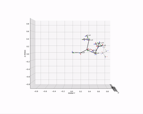
Plotting the output reveals valid mapping (it works!):
Implications
This approach allows for the generation of all possible solutions for kinematic chain mapping, and since the problem is kinematically underdetermined it may allow for the development of an objective function for optimization according to kinematic constraints of a system (e.g. joint degrees of freedom and range of motion).
The full code is available here.