
Non-uniqueness of the Euler axis in vector mapping
The 3D rotation group
This post requires some background theoretical knowledge of the 3D rotation group, or the special orthogonal group in three dimensions (SO(3)). This is an area of Linear Algebra in which special orthogonal matrices are used in three-dimensional Euclidean space. This group is widely used for representing object orientations.
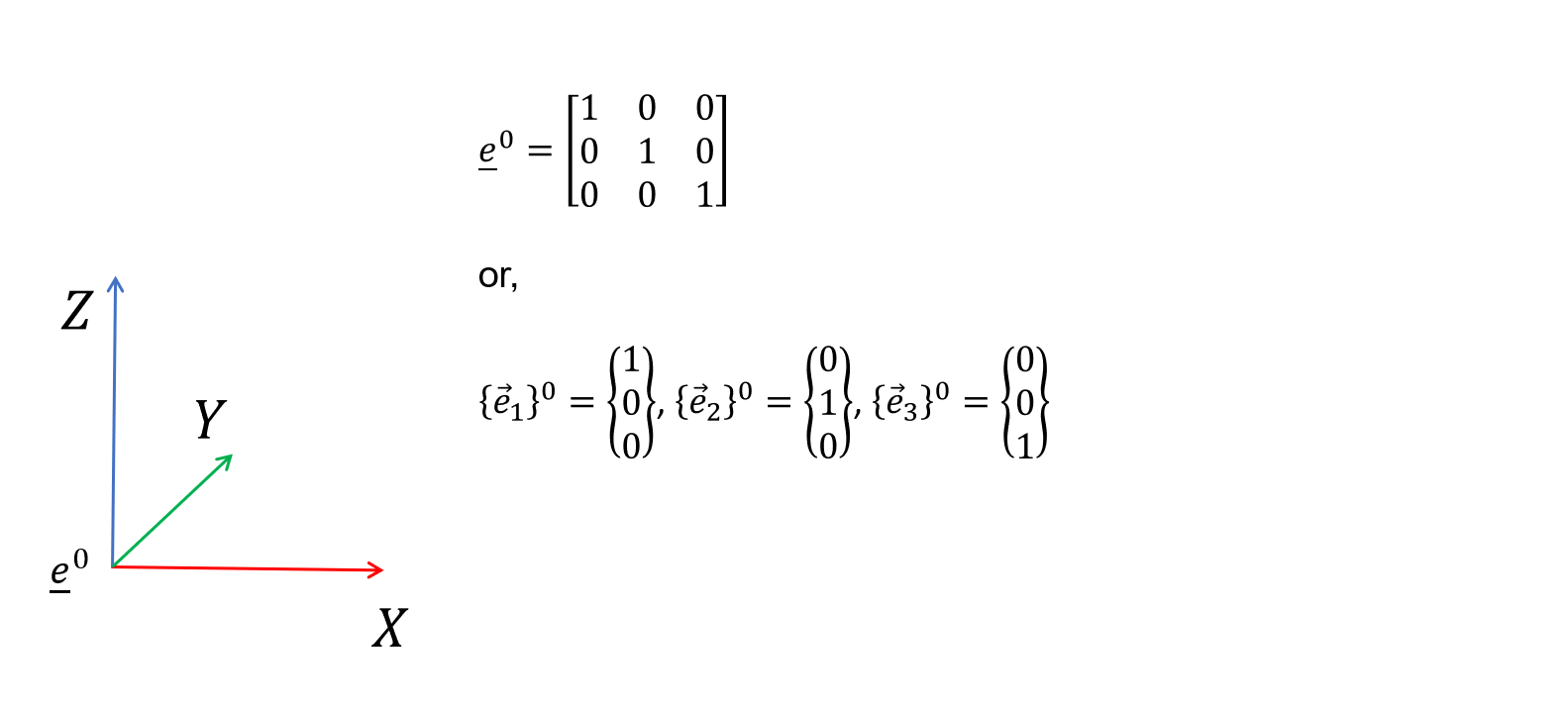
For this task, basis vectors are used to describe the directions of the cardinal axes of the object’s local coordinate system. For example, for object ‘0’ the local coordinate system can be described as follows using basis vectors; in this case the object is alligned with the global coordinate system, so the basis vector system is equal to the identity matrix (I), and each of the basis vectors ({e1}0, {e2}0, and {e3}0) extend 1 unit from the origin along each of the cardinal axes.
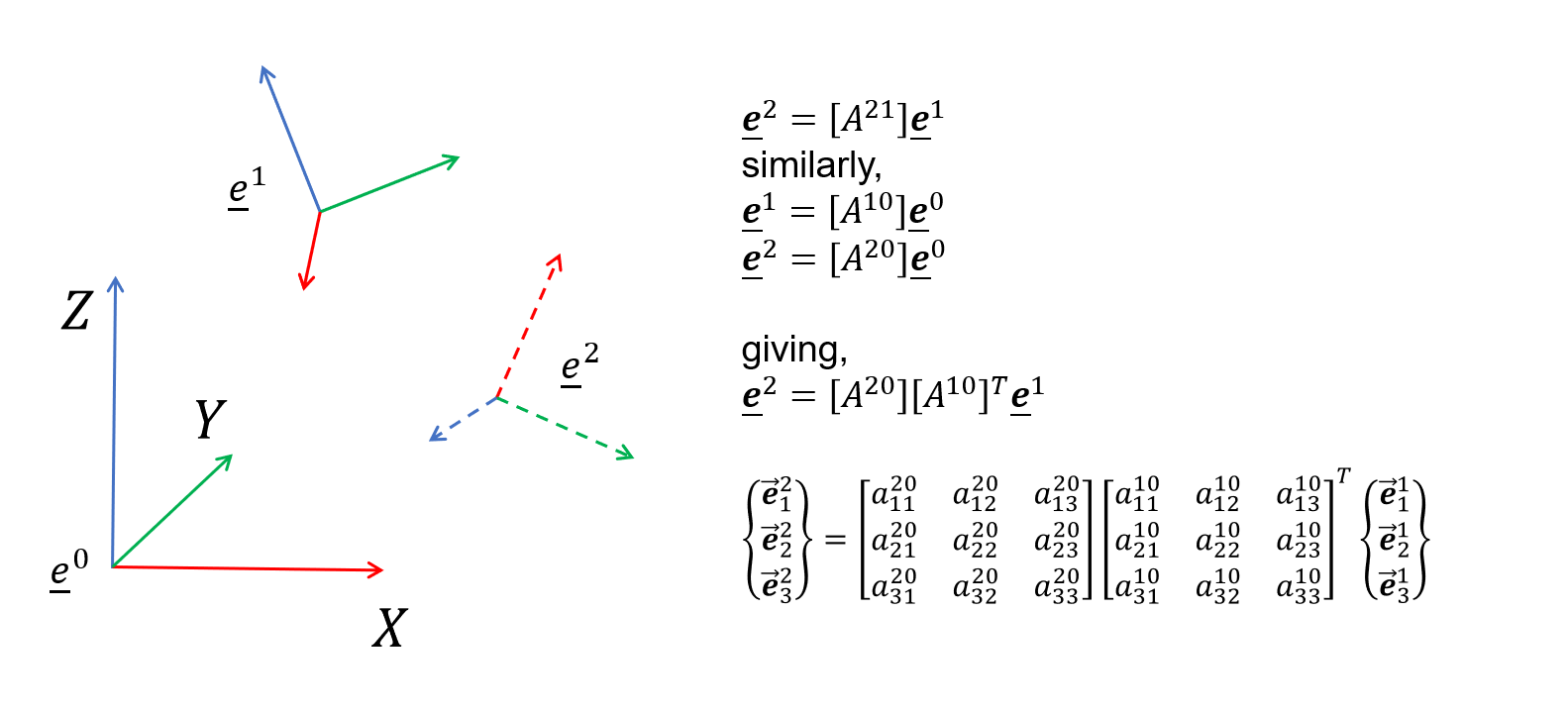
Furthermore, the orientation of one coordinate system represented using basis vector e2 can be represented wrt. another coordinate system e1 by multiplying the latter by a 3x3 rotation matrix [A21]. If we know the orientations of both of these coordinate systems wrt. a 3rd coordinate system e0, i.e. the global coordinate system, then we can find [A21].
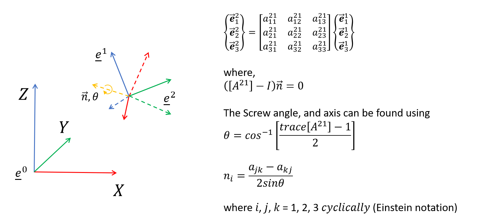
Euler’s rotation theorem states that, in three-dimensional space, any displacement of a rigid body such that a point on the rigid body remains fixed, is equivalent to a single rotation about some axis that runs through the origin of the coordinate system. This axis is called the Euler axis, or the Screw axis.
Mapping of two vectors
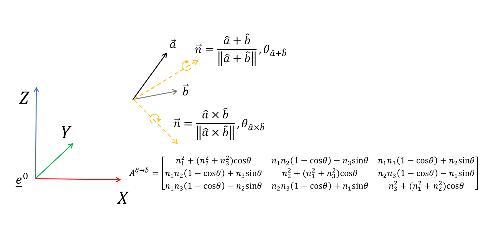
Now, consider the case where instead of having two complete coordinate systems represented by basis vectors, we only have two vectors a and b, which we want to use to represent a rotation between the two coordinate systems. Clearly, there will not be a unique solution to this problem so we need to define the Screw axis about which we rotate.
Two obvious candidate axes that can be chosen for this are:
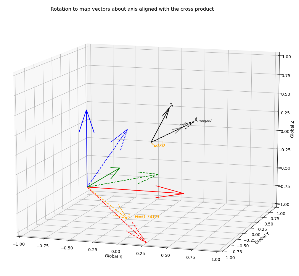
- the cross product of the vectors, which will be mutually perpindicular to both a and b, or
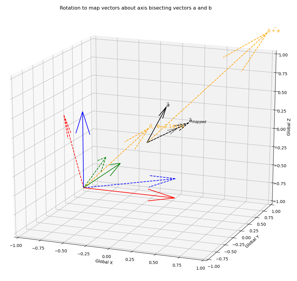
- the sum of the normalised vectors a and b, which symmetrically bisects a and b.
Choosing:
a=[0.1,0.3,0.4]
b=[0.3,0.1,0.2]
Implementation of cross product approach (axb):
def Vector_mapping_cross_product(vec1, vec2):
    """ Calculate the rotation matrix that maps vector a to align with vector b about an axis aligned with the cross product"""
    a, b = (vec1 / np.linalg.norm(vec1)), (vec2 / np.linalg.norm(vec2))
    n = np.cross(a, b) / np.linalg.norm(np.cross(a, b))
    adotb=np.dot(a, b)
    rotation_matrix = np.array([[n[0]**2+(n[1]**2+n[2]**2)*(adotb),n[0]*n[1]*(1-adotb)-n[2]*np.linalg.norm(np.cross(a, b)),n[0]*n[2]*(1-adotb)+n[1]*np.linalg.norm(np.cross(a, b))],
                                [n[0]*n[1]*(1-adotb)+n[2]*np.linalg.norm(np.cross(a, b)),n[1]**2+(n[0]**2+n[2]**2)*(adotb),n[1]*n[2]*(1-adotb)-n[0]*np.linalg.norm(np.cross(a, b))],
                                [n[0]*n[2]*(1-adotb)-n[1]*np.linalg.norm(np.cross(a, b)),n[1]*n[2]*(1-adotb)+n[0]*np.linalg.norm(np.cross(a, b)),n[2]**2+(n[0]**2+n[1]**2)*(adotb)]])
    return rotation_matrix
Implementation of bisecting vector approach (norm(a)+norm(b)):
def Vector_mapping_bisect(vec1, vec2):
    """ Calculate the rotation matrix that maps vector a to align with vector b about an axis aligned with norm(a) + norm(b)"""
    a, b = (vec1 / np.linalg.norm(vec1)), (vec2 / np.linalg.norm(vec2))
    n = (a+b) / np.linalg.norm(a+b)
    θ = math.pi
    rotation_matrix = np.array([[n[0]**2+(n[1]**2+n[2]**2)*(np.cos(θ)),n[0]*n[1]*(1-np.cos(θ))-n[2]*np.sin(θ),n[0]*n[2]*(1-np.cos(θ))+n[1]*np.sin(θ)],
                                [n[0]*n[1]*(1-np.cos(θ))+n[2]*np.sin(θ),n[1]**2+(n[0]**2+n[2]**2)*(np.cos(θ)),n[1]*n[2]*(1-np.cos(θ))-n[0]*np.sin(θ)],
                                [n[0]*n[2]*(1-np.cos(θ))-n[1]*np.sin(θ),n[1]*n[2]*(1-np.cos(θ))+n[0]*np.sin(θ),n[2]**2+(n[0]**2+n[1]**2)*(np.cos(θ))]])
    return rotation_matrix
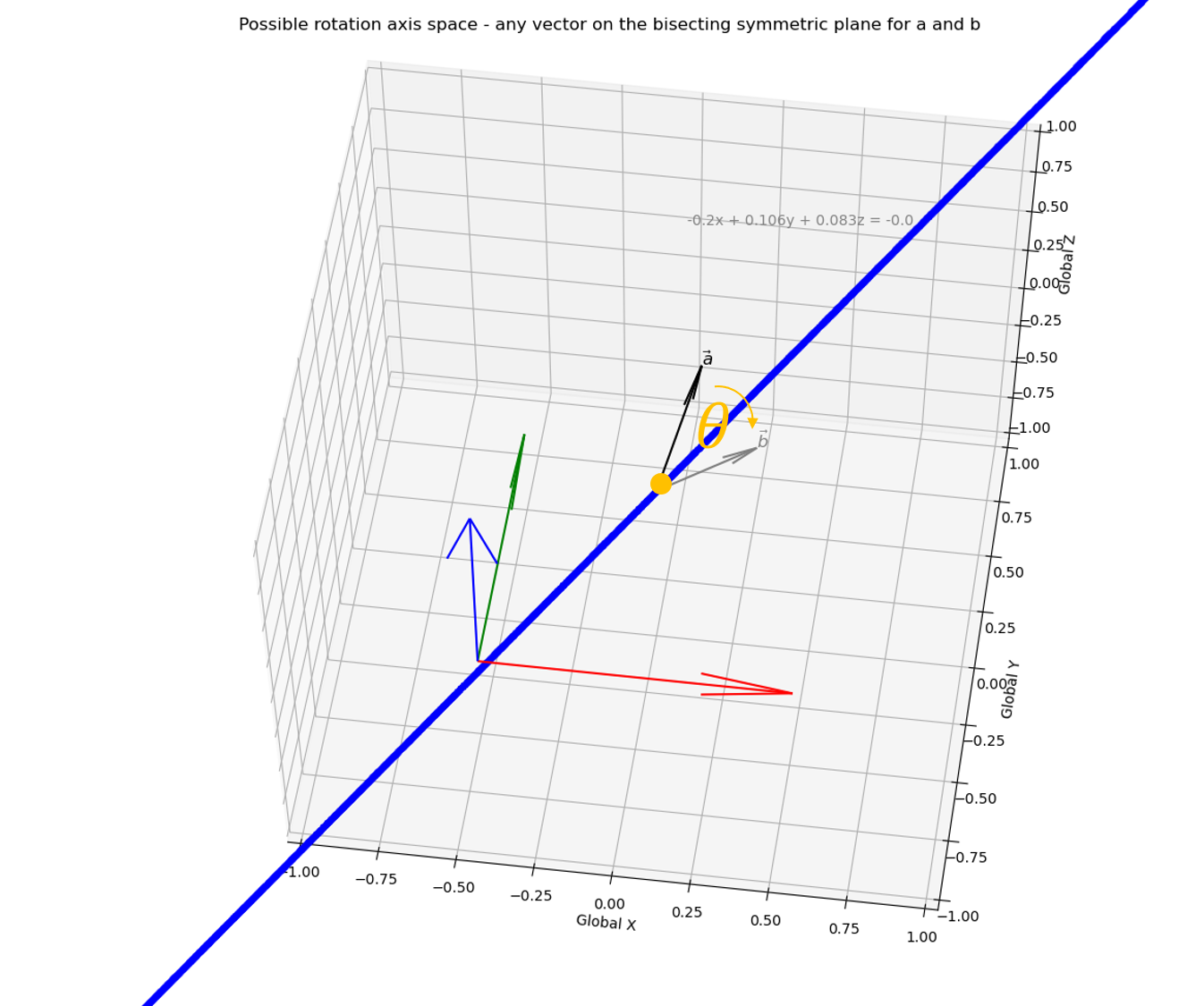
Now, we can use the two points obtained from the a+b approach and the axb approach along with the origin to define the plane that contains all possible rotation axes.
Or, more appropriately, we can define the Euler axis space as all unit vectors on the plane.
The axis-angle combination can be visualised by looking down the chosen axis to the origin - with the projection of the vectors a and b onto this plane the required angle becomes clear. This rotation can be visualised as a rotation of a right circular cone about its axis, where projections of vectors norm(a) and norm(b) lay on the surface of the base pointing outwards from the centre (i.e. the origin) to the directrix, and n points outwards from the centre of the base to the apex.
More formally, first choose two points which we know are on the Euler axis space.

Use these points to define the Euler axis space.

Project vectors norm(a) and norm(b) to lay on the base of a cone with the Euler axis as the cone’s axis.

The angle between these projected vectors is the Euler/Screw angle.

Now, we can formulate the all possible rotation matrices representing all possible Euler axis-angle combinations, i.e. the Euler axis-angle solution space (EAS).

Implementation of the devised approach:
def Vector_mapping_Euler_Axis_Space(vec1, vec2):
    """ Calculate all rotation matrices that map vector a to align with vector b"""
    a, b = (vec1 / np.linalg.norm(vec1)), (vec2 / np.linalg.norm(vec2))
    p1 = np.array([0,0,0])
    p2 = b / np.linalg.norm(b) + (a / np.linalg.norm(a))
    p3 = np.cross(a, b) / np.linalg.norm(np.cross(a, b))
    # create a list of candidate Euler axes (discritised to 1 degree)
    n=[]
    for i in range(0,360,1):
        α=np.radians(i)
        x_α=p1[0]+np.cos(α)*(p2[0]-p1[0])+np.sin(α)*(p3[0]-p1[0])
        y_α=p1[1]+np.cos(α)*(p2[1]-p1[1])+np.sin(α)*(p3[1]-p1[1])
        z_α=p1[2]+np.cos(α)*(p2[2]-p1[2])+np.sin(α)*(p3[2]-p1[2])
        n_α=[x_α,y_α,z_α]
        n.append(n_α / np.linalg.norm(n_α))
    # project vectors to form a cone around the Euler axis, and determine required angle for mapping
    rotation_matrices=[]
    Euler_axes=[]
    Euler_angles=[]
    for i in range(len(n)):
        Euler_axes.append(n[i])
        a_α, b_α = (np.cross(a,n[i]) / np.linalg.norm(np.cross(a,n[i]))), (np.cross(b,n[i]) / np.linalg.norm(np.cross(b,n[i])))
        θ = np.arccos(np.dot(a_α,b_α))
        θ = θ*np.sign(np.dot(n[i], np.cross(a_α,b_α)))
        Euler_angles.append(θ)
        if θ != θ: # if θ is NaN
            rotation_matrices.append(np.array([[ 1, 0, 0],
                                               [ 0, 1, 0],
                                               [ 0, 0, 1]]))
        else:
            rotation_matrices.append(np.array([[n[i][0]**2+(n[i][1]**2+n[i][2]**2)*(np.cos(θ)),n[i][0]*n[i][1]*(1-np.cos(θ))-n[i][2]*np.sin(θ),n[i][0]*n[i][2]*(1-np.cos(θ))+n[i][1]*np.sin(θ)],
                                               [n[i][0]*n[i][1]*(1-np.cos(θ))+n[i][2]*np.sin(θ),n[i][1]**2+(n[i][0]**2+n[i][2]**2)*(np.cos(θ)),n[i][1]*n[i][2]*(1-np.cos(θ))-n[i][0]*np.sin(θ)],
                                               [n[i][0]*n[i][2]*(1-np.cos(θ))-n[i][1]*np.sin(θ),n[i][1]*n[i][2]*(1-np.cos(θ))+n[i][0]*np.sin(θ),n[i][2]**2+(n[i][0]**2+n[i][1]**2)*(np.cos(θ))]]))

    return Euler_axes, Euler_angles, rotation_matrices
This function outputs valid mapping for all Euler axes on the plane (it works!):
for,
a=[0.1,0.3,0.4]
b=[0.3,0.1,0.2]
for,
a=[0.1,0.3,0.4]
b=[-0.3,-0.1,-0.2]
Implications
With a lack of complete basis vector representation for the two coordinate systems, there are an infinite number of rotation matrices, or axis-angle combinations that can be applied to achieve a desired vector mapping. However, here I have demonstrated that candidate Euler/Screw axes are constrained to be on the plane that bisects the vectors, such that the normalised vectors are symmetric to the plane. With this knowledge we can programatically solve for all possible vector mapping solutions.
The full code is available here.